


 nueva página del texto (beta)
 Inglés (pdf)
 Artículo en XML
 Referencias del artículo
 Enviar artículo por email
 Citado por SciELO
  Similares en
SciELO
Similares en
SciELO 
 Permalink
1 Introduction and Related Work
sec01) Since some decades ago, the performance of evolutionary computation has significantly improved, enabling the resolution of various optimization problems. From basic procedures to very elaborate hybrid methods, all of them efficiently address most NP-hard issues. Normally, any optimization algorithm, specifically evolutionary algorithms, involves creating a population of solutions, selecting certain members based on their aptitude, reproducing them to generate offspring, and repeating this process until the best solution is obtained. We are used to developing optimization algorithms using the same procedures, such as initial population, selection, crossover, mutation, and replacement. This is because we perceive the survival of the species as a well-defined process. Although almost all optimization algorithms share this feature, there are other algorithms inspired by different natural processes, such as particle swarm optimization and artificial immune systems. In fact, some evolutionary algorithms, particularly ’evolutionary programming’ and older varieties of evolution strategy, do not use recombination at all [13]. Therefore, there are alternative possibilities for creating optimization algorithms that are not inspired by the aforementioned population-based procedures of evolutionary algorithms.
An example is asexual living beings. Asexual reproduction enables living beings to transmit their genetic information to their descendants without the union of information (gametes) from individuals. In real life, jellyfish, corals, and sea sponges are examples of the absence of recombination.
There are already algorithms composed of various populations that do not communicate with each other but rather evolve independently. The research by Absi et al [1] falls into this category.
In this paper, we propose the absence of recombination and the idea of no communication among members of the population.
In this research, the concept of competition among members of the population is not considered. On the contrary, members of the population participate and cooperate to build a global aptitude for the entire population. The global aptitude is obtained through the contribution of all members, without individual fitness values. Members are not selected for specific purposes, and offspring can be generated through either classical procedures or alternative methods, depending on each researcher’s approach. The replacement process between offspring and parents is decisive, with the population exhibiting the best fitness surviving and completely replacing the less fit population. This process can be likened to a binary tournament between parents and offspring. Given these characteristics, we refer to this algorithm as the Cooperative Algorithm (CoopA), utilized to solve the truck and trailer routing problem (TTRP), which is an NP-hard issue.
Normally, in almost any evolutionary algorithm, each member of the population represents a solution, and aptitude is computed based on its codification. However, in CoopA, it is not possible to compute aptitude based solely on a member’s codification because each member has only partial information about the solution. All members of the population possess partial information. Therefore, cooperation among members is essential to obtain an aptitude for the entire population. This method of computing fitness represents a gap in the literature and warrants further investigation.
The Truck and Trailer Routing Problem (TTRP) is particularly suited for resolution using the novel CoopA scheme. In essence, the TTRP involves delivering products to customers using a combination of trucks and trailers. Vehicles depart from a central depot to traverse various routes, with each vehicle returning to the depot upon completing its journey.
Beyond capacity constraints, the TTRP incorporates operational restrictions, such as limited trailer access at certain customer locations. This limitation arises due to factors like narrow spaces for maneuvers, traffic restrictions, and other considerations. Consequently, vehicles must be parked elsewhere, trailers unhitched, and the journey continued using only the truck before reaching customers with restricted trailer access. After product delivery, the truck returns to retrieve the trailer before continuing its journey.
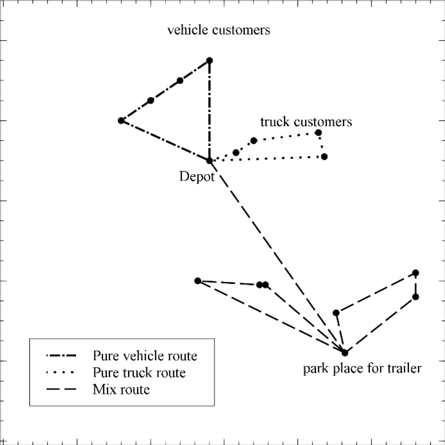
The unique considerations outlined above give rise to three main types of routes. The first type exclusively employs trucks for product delivery, termed ’truck routes.’ The second type, called ’vehicle routes,’ involves using both the truck and trailer for customers with unrestricted access. The third type, ’mix routes,’ also employs both the truck and trailer but requires unhitching when encountering customers with maneuvering restrictions.
Customers who only permit access to trucks at their facilities are labeled ’truck customers,’ while those allowing access to both trucks and trailers are termed ’vehicle customers.’ In the TTRP, it is possible to park and unhitch the trailer at any vehicle customer location before delivering products to truck customers on the trip, see Fig 1.
Finally, the main objective is to select a set of routes, minimizing the total distance traveled, to efficiently deliver products to all customers.”
Based on the characteristics of the TTRP, it is suitable to apply the CoopA. The purpose is to build many routes as possible, and all of them are built through the information of the members of the population. Each member participates and cooperates with a set of routes in order to find and select the best of them, i.e., of minimum total distance. Thus, each member has only partial information of the solution, i.e., a set of routes. Therefore, the fitness of the population is obtained by choosing from the routes of minimum total distance.
Currently the majority of methods to resolve vehicle routing problems use a conventional mechanism to build solutions, i.e., group customers in a route, and then sequence the route. It is commonly named ‘cluster-first route-second’. The constraints of the problem being analyzed are considered to group customers.
Prins et al [15] cited contributions of this approach for vehicle routing optimization problems, such as [19, 8, 23] cited important contributions for the TTRP using this approach. Examples of applications in real-world situations are found in [5, 7, 9, 2, 20, 22, 28]. However, for two decades, an alternative approach has had increasing acceptance, i.e., the ‘route-first cluster-second’ mechanism. This relatively new approach has led to successful methods for routing problems. It is due to its flexibility and efficiency. Such properties have let to resolve the TTRP too. Again in [15] and [23] cited the most relevant papers in this category, such as [3, 10, 14, 16, 17, 24, 25, 23]
In the route-first cluster-second, generally each solution for the TTRP, is represented for a permutation of vertices. Therefore, after the split-phase, a fitness is obtained for that solution. In this research, also we adopt the route-first cluster-second approach, but we differ in the split-phase to build routes. This dissimilarity permits to represent of a member of the CoopA population as a route. Thus, each route is a member of the population in the core of the CoopA. It is then clear that each route only contains partial information of the solution and it is necessary to consider all the routes to generate a population fitness.
Basically, the TTRP’s current research is focused on the use of heuristics and metaheuristics. The tabu-search algorithm is used to tackle the TTRP in [4]. With tabu search, the author allocates customers to routes at the beginning, followed by an insertion heuristic. Scheuerer employs two heuristics in [18] to develop initial solutions, and later the solutions are improved through tabu search. In [18] the authors address the TTRP through sequential heuristics. First, assigns customers to valid routes, and then defines the sequence of each route In [18]. Yu et al tackle the TTRP by an ant colony system to build feasible solutions, and then these solutions are improved by a process improvement for each solution.
In [11], Lin et al detail a heuristic based on SA technique for the TTRP. In [28] Authors extends the idea to address the time window constraints.
Villegas et al in [23] detail a hybrid Greedy Randomized Adaptive Search Procedure (GRASP) with Variable Neighbourhood Search (VNS) heuristic for the TTRP. In [24] Villegas et al coupled this heuristic with a set-partitioning formulation to tackle the same problem.
If time windows for delivery exist, and the option of load transfer between truck and trailer is required, the paper of Derigs et al [6] is suitable when we need to analyze the Rich Vehicle Routing Problem (RVRP). The study details a flexible hybrid approach, which is based on local search and large neighborhood.
In [1], Absi et al propose an evolutionary algorithm composed of multiple populations that evolve independently, without communication, to solve the TTRP (Truck and Trailer Routing Problem).
In [12] Maghfiroh and Hanaoka solve a dynamic truck and trailer routing problem for last mile distribution in disaster response by a modified simulated annealing algorithm with variable neighborhood search for local search. The fitness in this research is the total travel time. For dealing with the stochastic and dynamicity of the problem, a dynamic simulator is added to the framework to incorporate new requirements of the customers.
In [27] Wang et al detail a bat algorithm (BA) to tackle the TTRP. The procedure uses five different neighborhood structures as part of local search strategy. Moreover, to preserve diversity, a self-adaptive (SA) tuning strategy is used in the proposed algorithm.
In [29] Yuan et al tackle the TTRP by a Backtracking Search Algorithm (BSA). The algorithm uses four types of route improvement to produce offspring, and a T-sweep heuristic to build the initial population.
Although diverse methods and strategies have been used to solve the TTRP, this paper contributes to the state of the art by the use of the idea of absence of recombination. We adopt the idea of no communication among members of the population.
2 A Set-Partitioning Formulation for the TTRP
Previously we discuss the possible routes that can be built in the TTRP, i.e., truck routes, vehicle routes, and mix routes. Also, erstwhile we refer to truck customers, and vehicle customers. Then we can establish binary parameters for each sort of route. It means:
Parameters:
|
Set of feasible truck routes. |
|
Set of feasible vehicle routes. |
|
Set of feasible mix routes. |
|
Set of truck customers. |
|
Set of vehicle customers. |
|
represents the total distance of the truck route |
|
represents the total distance of the vehicle route |
|
represents the total distance of the mix route |
Variables:
The objective function (1) consists of the first part that corresponds to the total distance of truck routes, the second part represents the total distance of vehicle routes, and the third part is the total distance of mix routes. Constraints (2) assure that each vehicle customer is visited exactly once; whereas, constraints (3) assure that each truck customer is visited exactly once by a truck route or by a mix route.
3 CoopA Framework
3.1 Route-First Step
A permutation representation is built to execute the route-first step. The CoopA uses five different procedures to build permutation representations, i.e., trips. All the procedures are well-known techniques in the literature.
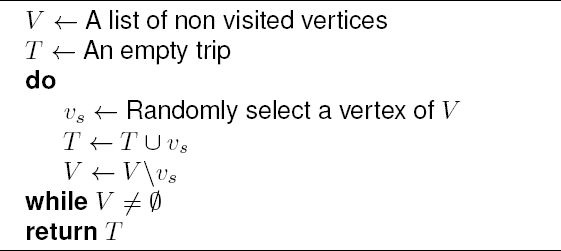
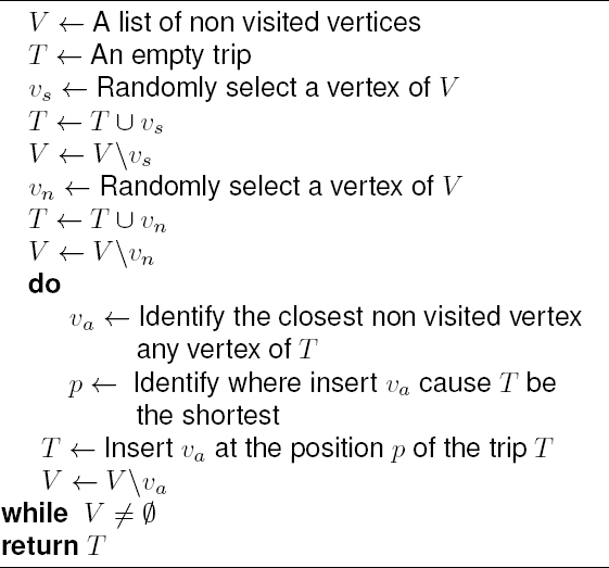
3.1.1 Random Insertion
The first one, it is a random procedure, where all the vertices are positioned on the trip randomly, i.e., the procedure randomly selects a vertex from a list of not visited vertices and inserts it in the trip. Update the list of not visited vertices, and repeat the procedure until all the vertices are included in the trip. The Algorithm 1 shows the random insertion procedure.
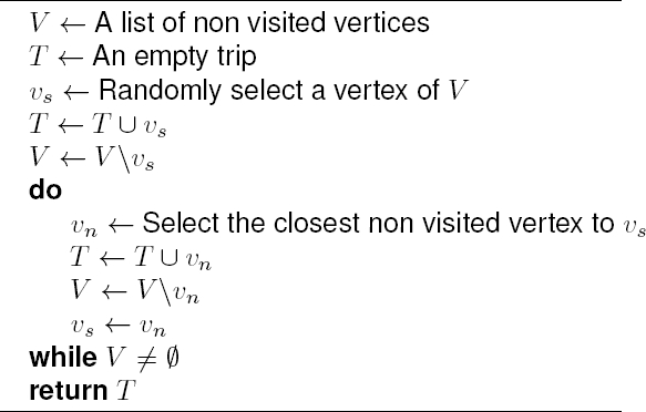
3.1.2 Nearest Neighbour Procedure
The second, the nearest neighbor procedure starts at one vertex (randomly selected from a list of not visited vertices and inserts it in the trip), update the list of not visited vertices, identifies the closest unvisited vertex, and inserts the closest unvisited vertex to the trip, again update the list of not visited vertices. It repeats until every vertex has been visited. Algorithm 2 shows the Nearest neighbour procedure.
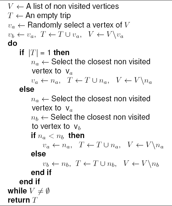
3.1.3 Adaptative Nearest Neighbor Procedure
The third, the nearest neighbor procedure from both end-points, where it starts with a vertex chosen randomly. Then, it continues with the nearest unvisited vertex to this vertex. We will have two end vertices. We add a vertex to the trip such that this vertex has not visited before and it is the nearest vertex to these two end vertices. We update the end vertices. It ends after visiting all the vertices. Algorithm 3 shows the Adaptative nearest neighbour procedure.
3.1.4 Nearest Insertion Procedure
The fourth, the nearest insertion procedure, where it begins with two vertices. It then repeatedly finds the vertex not already in the trip that is closest to any vertex in the trip, and places it between whichever two vertices would cause the resulting trip to be the shortest possible. It stops when no more insertions remain. Algorithm 4 shows the Nearest insertion procedure.
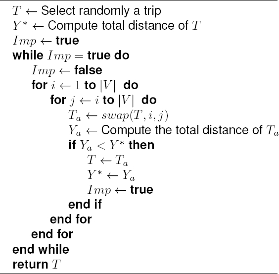
3.1.5 2-Opt Procedure
Finally, the fifth, the 2-Opt procedure proposed by Croes (1958), where it originates from the idea that trips with edges that cross over are not optimal. 2-Opt will consider every possible 2-edge swap, swapping 2 edges when it results in an improved trip. Algorithm 5 shows the 2-Opt procedure.
3.2 Cluster-second step
Each trip, obtained in the previous step, is split as many feasible routes as possible. For that purpose, three variants are used to build feasible routes.
3.2.1 Building Feasible Truck Routes
In this case, we read each trip from left to right. Let a trip
3.2.2 Building Feasible Vehicle Routes
The process is very similar than the previous one. The main difference is found in the capacity of the vehicle, which is no longer
3.2.3 Building Feasible Mix Routes
The process starts reading the trip as the previous ones. The capacity of the vehicle is
The next step is to verify if the route, already built, contains at least one truck customer. If so then, we confirm that the first vertex on the route be a vehicle customer. If so then, the route is a mix route, and we park and unhitch the trailer is that first vertex. If not then, the route is unfeasible and it is discarded. The process continues reading the rest of the trip, and it finishes when we have already analyzed all the vertices on the trip.
All the routes built by these three variants are members of the population, in the CoopA framework. All the routes are considered to find a fitness for the population.
3.3 Total Distance Computing
For each route built by any of the three aforementioned variants, a total distance is computed. The total distance for the truck routes and the vehicle routes is easily computed because it corresponds to a single tour, without forgetting that the route leaves the depot and returns at the end. The total distance for the mix routes is computed considering that the trailer is unhitch at the first vehicle customer location on the route, after that the truck visits one or more customers on the route, probably the truck has to come back to the parking place of the trailer to transfer product between the trailer and the truck, and continue the tour until satisfying pending customers. We emphasize that the route leaves the depot, sometime the truck has to return to hitch the trailer, and finally the vehicle goes back to the depot at the end.
3.4 Fitness of the Population
The mathematical model, detailed in Section II, is applied to minimize the total distance of the solution, i.e., the fitness of the population. This model considers all the routes built in Section III-B, the total distance of each route computed in Section III-C., to identify the minimum, and know which routes are elected.
3.5 Offspring Population
Again, we create trips by five different procedures. Four of them, have been previously detailed in Section III-A, i.e., the nearest neighbor technique, the nearest neighbor technique from both end-points, the nearest insertion technique, and the 2-Opt technique.
The fifth procedure is the partially mapped crossover, called PMX genetic operator. Here, we select randomly two trips, obtained in Section III-A, and we apply the PMX operator to produce one new trip. The process detailed in III-B, is repeated to produce feasible routes that we consider as the offspring population in the CoopA framework. The processes III-C, and III-D, are repeated to know the fitness of the offspring population.
3.6 Replacement
Although the population with the best fitness survives, the best trips of both populations are preserved to build feasible routes in the next generation.
The parameters used are detailed below.
The CoopA framework is provided in Algorithm 6

4 Results and Comparison
The CoopA is compared with other evolutionary algorithms in order to show its performance. The comparison is done using the algorithm detailed by Derigs et al in [6], the simulated annealing heuristic designed by Maghfiroh and Hanaoka in [12], and the bat algorithm presented by Wang et al [27]. All these algorithms were implemented following the available information. The proposed approach is applied to Chao’s 21 TTRP benchmark problems in [4] available on the web http://140.118.201.170/ttrp/
The Chaośs benchmark problems include
— On the first line of each instance, the capacity of the trucks, the capacity of the trailers, and the available number of the vehicles.
— From the second line of each instance to the end, the information of each customer, i.e., the number of customer and depot, the X coordinate, the Y coordinate, the demand, and availability to accept the complete vehicle in its location.
Fig. 2 details the performance for each algorithm.
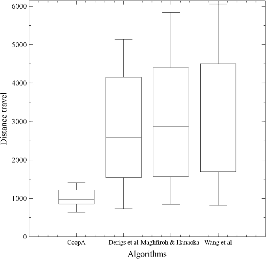
Based on Fig. 2, the dispersion of the results is less in the CoopA than others. It is due to the replacement procedure, detailed in section 3-F., keeps the best fitness over all the iterations, and the average of each generation cannot be far away from the best solution because the most offspring are built by the same procedures than the parents.
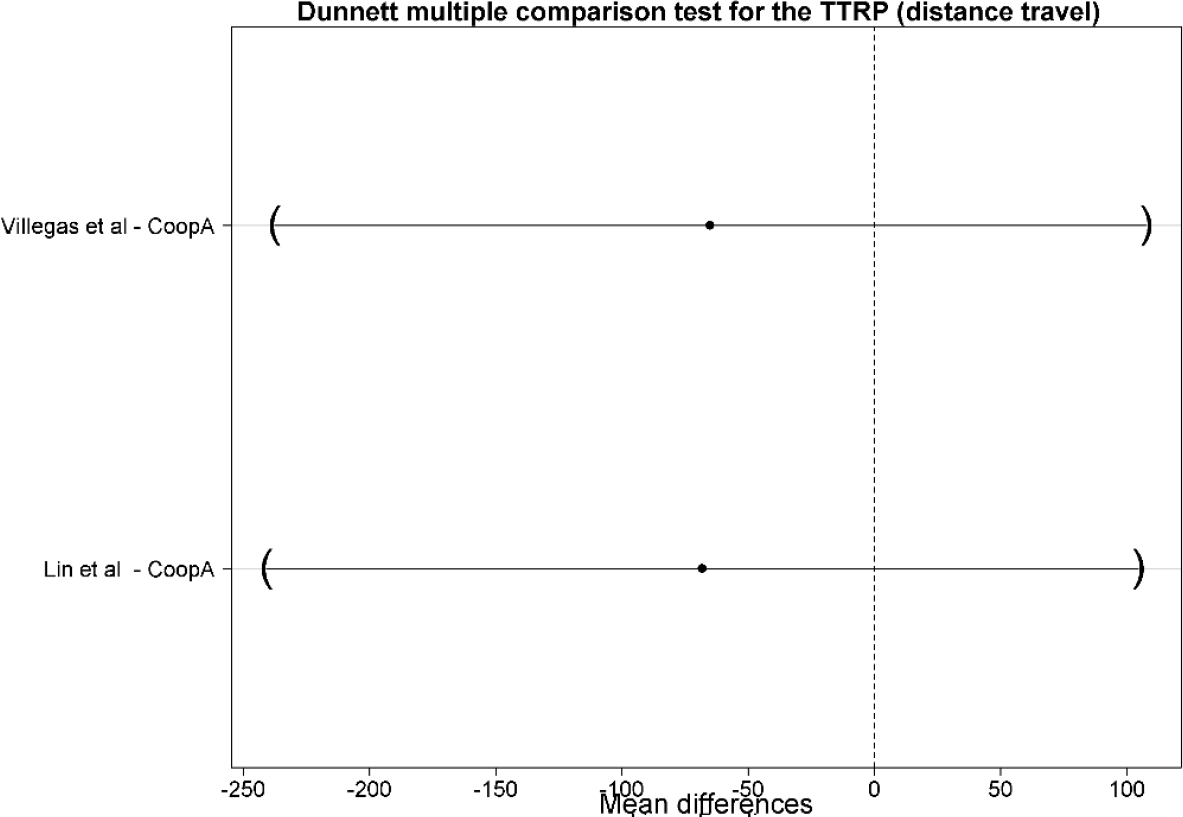
In addition, another comparison is presented in Fig. 3. It is using the algorithm proposed by Lin et al. in [11], and the procedure shown by Villegas et al. in [24] for comparison with the CoopA scheme. The results of these algorithms were taken directly from the available literature, and the same dataset (Chao’s 21 TTRP benchmark problems) was used in this comparative.
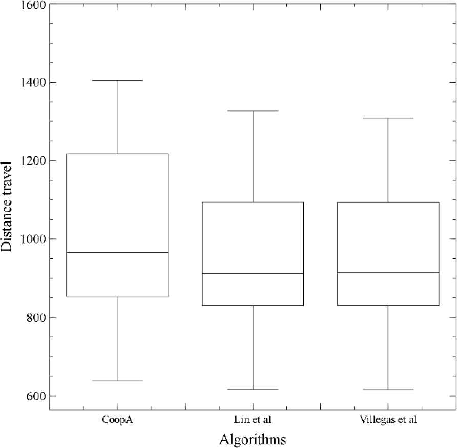
Based on Fig. 3, the dispersion of the results is very similar among the algorithms. The performance of CoopA is competitive. It is due to the large number of routes built in each instance. We devised procedures, detailed in section III-B., to tackle the most drawback of the set-partitioning model for the TTRP, i.e., the structure of mix routes that normally are resolved by column generation and branch-and-price methods (Drexl, 2011). Furthermore, in this research, we do not use any auxiliary graph to build feasible routes.
A Dunnett test [21] is done to identify if there exist statistically significant difference between CoopA and the other methods. The CoopA is competitive, there no exist statistically significant difference (see Fig. 4). It means that CoopA is a new approach to continue developing.
Villegas et al in [26] indicated that the set-partitioning model for the TTRP is often impractical. It is due to the huge number of feasible routes, and since it is impossible to compute all of them, the CoopA scheme builds a considerable number of them to tackle the aforementioned drawback. Table 1 details the number of routes computed by the CoopA scheme, and the best solution founded for the instance number one.
5 Conclusions and Future Research
The CoopA scheme detailed above, is suitable to tackle the TTRP. It is a well-known NP-hard issue. The main drawback of the set-partitioning model, i.e., the inability to compute all the routes, is cleverly resolved by devised procedures, and detailed in section III-B. Based on the results shown in section IV, the CoopA scheme is competitive. It was not necessary to incorporate auxiliary graphs to create feasible routes for those possible mix routes.
The set of instances used in the comparison are considered benchmarking. Therefore, the use of the Dunnett test is clearly justified and forceful. The performance of the CoopA scheme should be taken into account in the literature.
The proposal of the CoopA, i.e., considers all the members of the population to obtain a fitness for the all the population is substantial. Each member participates and cooperates to identify the fitness of the population. It is obtained by choosing from the routes of minimum total distance.
Although each member of the CoopA scheme only has partial information of the solution for the population, it is not a drawback for the CoopA scheme, on the contrary, this enriches its performance by consider many routes in the solution (see Table 1).
As future work, other greedy procedures should be implemented to create trips, to help the CoopA to find more suitable routes. In addition, other procedures should be incorporated to get offspring, to enhance the performance of the CoopA. Other optimization problems should be resolved by the CoopA scheme, in order to confirm its performance. Finally, application tools for users should be implemented in practice and real life situations using this approach.

