


 nueva página del texto (beta)
 Inglés (pdf)
 Artículo en XML
 Referencias del artículo
 Enviar artículo por email
 Citado por SciELO
  Similares en
SciELO
Similares en
SciELO 
 Permalink
1 Introduction
In recent times, text documents have become the most essential resource for the user in daily life. Such documents show useful information in different formats (e.g., books, scientific/news articles, monographs, and social media comments) that satisfy users' requirements. Nevertheless, they grow exponentially on the Internet, causing an information overload. For this reason, the Automatic Text Summarization (ATS) seeks to solve this problem because it is considered the most recognized kind of text condensation [1].
Over the last two decades, several methods have been proposed in the ATS that generate summaries of different characteristics (single- and multi-document; extractive, abstractive, and hybrid; generic and query-based; monolingual, multilingual, and cross-lingual) [2]. However, the Evaluation of Text Summaries (ETS) is a complex task that requires exhaustive studies to determine suitable criteria to assess summaries [3].
According to Jones and Galliers [4], each evaluation method may be extrinsic or intrinsic. The extrinsic evaluation measures the usefulness of summaries in another task, such as document categorization, relevance assessment, and web search [5, 6]. On the other hand, the intrinsic evaluation focuses on the suitability of the summarization approach in terms of text quality and content analysis [7].
In other words, it analyzes the summary's content, coherence, and informativeness [8]. Most of these methods generally compare the content between a summary to be evaluated (candidate summary) and a set of summaries written by the human expert (human references).
Depending on the degree of human intervention, an evaluation method may be manual, semi-automatic, or automatic. Manual assessment involves human judgments to decide whether a summary shows the essential information from one or more documents. Nevertheless, this evaluation faces two drawbacks: (i) it is time-consuming, and (ii) several assessors are required to evaluate many summaries [8]. Considering the issues mentioned above, automatic evaluation has been proposed.
For this evaluation, ROUGE (Recall-Oriented Understudy for Gisting Evaluation) is the most representative package in the state-of-the-art that includes some measures, such as ROUGE-N, L, W, and S to evaluate the content of summaries [9]. However, these measures are inadequate when they do not have human references. Due to this situation, the ETS without human references has been proposed.
The ETS without human references has attracted attention since traditional methods are impractical and expensive. In this regard, ROUGE-C [10], LSA [7], and SIMetrix [11] have been proposed as methods that compare the candidate summary's content concerning its source document(s). These methods consider source documents as references because they contain enough information, providing helpful knowledge about the topic, but they are still far from manual assessment [12].
To solve this issue, previous studies have proposed the linear optimization of content measures through Genetic Algorithms (GAs) to improve automatic evaluation [3, 13]. The outcome of this research was SECO-SEVA, an evaluation package that combines 31 content measures derived from ROUGE-C, LSA, and SIMetrix. However, the GA's optimization assumes the presence of different levels of complexity in each evaluation measure.
In this paper, we propose a selection of content measures for the ETS without human references, using the GA. We assume that assigning a complexity value to each source document and measure may be a suitable indicator to estimate an adequate evaluation measure for each summary. For this, we have employed 13 complexity indexes known in the state-of-the-art and 31 evaluation measures used in [13].
The paper is organized as follows. In Section “Related Works”, we present a brief description of related works of this research. In Section “State-of-the-Art Evaluation Measures and Text Complexity Indexes”, we describe state-of-the-art evaluation methods and complexity indexes.
The proposed method is presented in Section “Proposed Method”. In Section “Experiments and Results”, we display the results of the proposed selection of measures and a comparison to other state-of-the-art methods. Finally, the conclusions and future works are drawn in Section “Conclusions and Future Works”.
2 Related Works
Over the last few years, several studies have been conducted to improve automatic evaluation. Some perform the linear optimization of measures through the Monte Carlo method [14], linear regression [15], and GA [13]. Other works employ single and ensemble learning classifiers that use evaluation measures as features to predict the score of summaries [16, 17].
Although such works seek the combination of evaluation methods to improve automatic evaluation, it does not always guarantee a better approximation toward human judgments. We assume this because if we include more perspectives to solve a problem, the complexity of the task is increased. This situation is similar to other Natural Language Processing (NLP) tasks.
In [18], García-Calderón et al. proposed a hybrid method based on a selection of Text Line segmentation (TLS) methods, using a complexity index called TLS-ICI (Text Line Segmentation Intrinsic Complexity Index). The TLS-ICI index is shown in Eq. (1), which is the average of four normalized subindexes that measure the amount of information presented in an individual interlinear space.
Let an image I composed of an interlinear space from a handwritten document; therefore, the complexity of such space is calculated using the Horizontal Projection Profile (HPP), the Vertical Projection Profile (VPP), the Histogram of Color of the Bitmap (HCB), and the Histogram of Color of the Ink (HCI):
Once the complexity of an interlinear space is calculated, it is estimated the overall complexity of a document according to Eq. (2), where
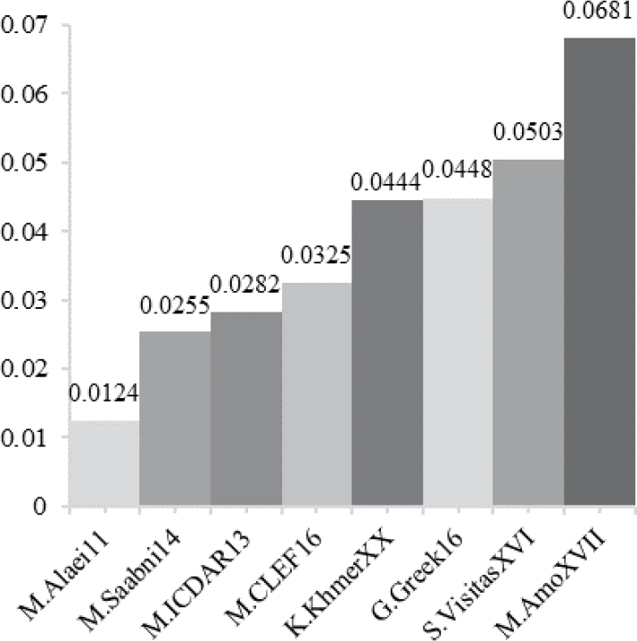
Based on TLS-ICI calculates the complexity of handwritten documents, it likewise provides an order of complexity to collections of documents. Such an order establishes that the first collections show lower complexities than the subsequent ones. For the experimentation stage, this order was obtained from eight collections of contemporary and ancient texts written in English, Spanish, Arabic, Chinese, Greek, Khmer, Persian, Bengali, Oriya, Kannada, and Nahuatl [19, 20, 21, 22, 23, 24, 25, 26].
Fig. 1 shows the average TLS-ICI for each collection. As observed, all collections are sorted from lower to higher complexity values. According to the collection, M.AmoXVII shows the highest complexity. Therefore, it would be expected that, in principle, the most sophisticated method performs best the task in this collection. On the other hand, collections of lower complexities (e.g., M.Alaei11 or M.Saabni14) should be analyzed by straightforward TLS methods.
In addition to collections, measuring the complexity of state-of-the-art TLS methods was also necessary. Based on this, the authors selected Ptak [20], Arvanitopoulos [27], García [28], and Arivazhagan [29] methods since they are considered the best ones for the TLS.
Afterward, the complexity of each method was calculated by the maximum complexity threshold with 95% of the accuracy of
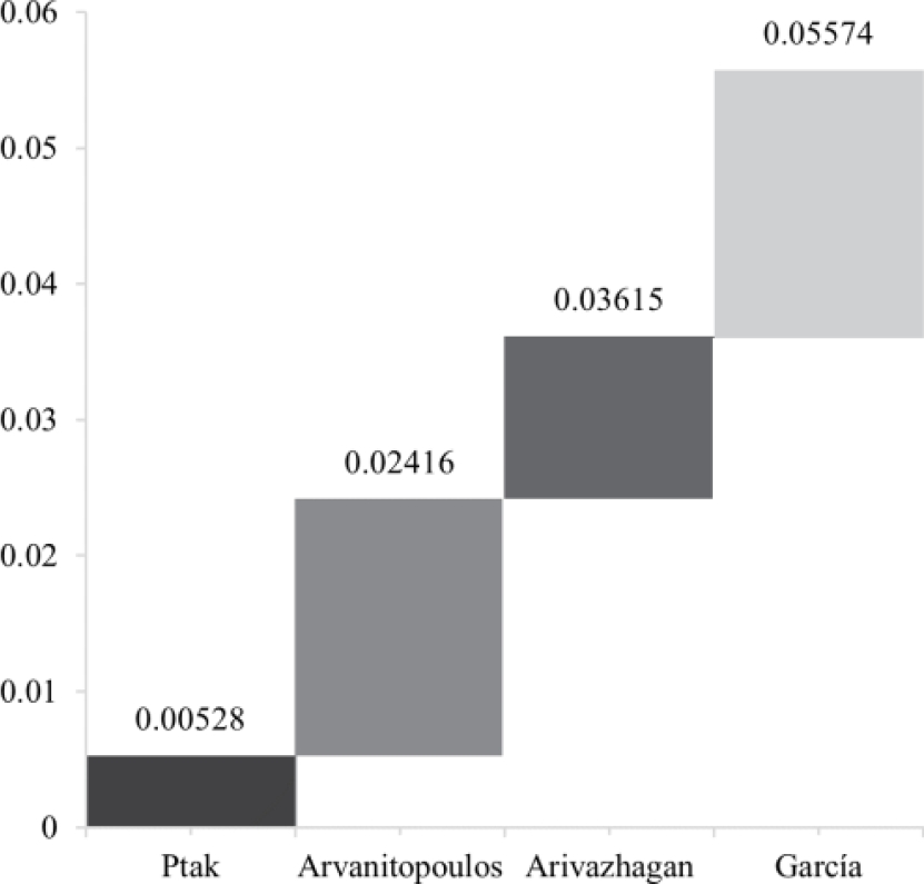
The García method displays the most increased complexity, which means this method can analyze more complex documents. Based on the values shown in Fig. 2, the complexity values of each TLS method were used to determine the ranges that each method should be selected, creating a Hybrid Method (
As observed, the
For instance, if a document obtains a
3 State-of-the-Art Evaluation Measures and Text Complexity Indexes
Content-based measures and text complexity indexes are two groups of measurements that help to estimate specific attributes of texts. While the first group is typically used to evaluate summaries with or without human references [30], the second group employs different formulas that estimate the degree of ease or difficulty a text can be understood according to its vocabulary [31], readability [32], or word morphology [33]. In this section, we briefly describe evaluation measures and text complexity indexes that are part of this study.
3.1 Evaluation Methods and Measures
The ETS without human references has been an active area of research in recent years since traditional methods are expensive and impractical.
Based on this, ROUGE-C, LSA, and SIMetrix have been proposed as methods that compare the content between summaries and their source document. Below, we briefly describe these methods and their underlying measures.
ROUGE-C. For automatic assessment, ROUGE is a well-known evaluation package of four measures (ROUGE-N, L, W, and S) that estimate the similarity between the automatic summary and its human references. For instance, ROUGE-N calculates the overlap of n-grams between the summary and its human references (
where
Unlike ROUGE, ROUGE-C employs source documents to measure their similarity concerning the automatic summary. Fig. 1 exhibits the differences between ROUGE and ROUGE-C. As observed, ROUGE measures receive human references and automatic summaries as model and test documents, respectively. On the contrary, ROUGE-C inverts the order of both documents, where the source document is used as a test, and the summary is used as a model.
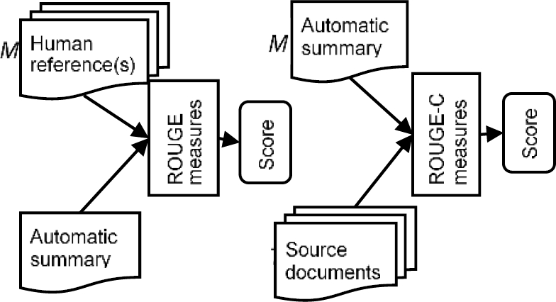
Based on the differences shown in Fig. 1m ROUGE-N, L, W, S, and SU4 measures can be adapted, generating the following variants: ROUGE-C-N, L, W, S, and SU4. As an example, the evaluation of ROUGE-N without human references is called ROUGE-C-N, which is formally defined in Eq. (5):
where
Latent Semantic Analysis (LSA). The LSA is a matrix processing method that represents, extracts and relates the contextual meaning of terms from a document in a “latent” semantic space [34]. For the ETS, the LSA evaluates summaries by measuring the contextual similarity between the summary and its source document(s) [7]. In general, the LSA consists of the following steps:
1 Preprocessing. The summary and its source document(s) are preprocessed by eliminating stopwords and performing stemming. After this, the remaining terms are grouped into n-grams of different lengths, preserving their order in sentences.
2 Represent input documents as matrices. The summary and its source document must be represented into two matrices
3 Singular Value Decomposition (SVD). The matrices
-
where
4 Matrix similarity calculation. Once the SVD has been performed, the resultant matrices of both documents are compared through Main Topic Similarity (MTS) or Term Significance Similarity (TSS). While MTS extracts and measures the similarity between the first left singular vector of the summary and source document, TSS extracts singular values and left singular vectors to measure the similarity between the summary and the source document.
Summary Input similarity Metrics (SIMetrix). SIMetrix is an evaluation package that employs 10 similarity and distance measures to evaluate summaries without human references [11]. Some measures are based on vector space similarity, word probability distributions, and topic signature words between the summary and the source document. However, the measures with the best correlation results derive from the Kullback-Leibler (
Divergence measures are based on the concept of probabilistic uncertainty or entropy [37], whose use was originally proposed to quantify the loss of information between two communication signals [38, 39]. Nevertheless, both measures were later proposed to measure the loss of information between the summary concerning its source document. Formally,
Although
where
where
On the other hand,
3.2 Text Complexity Indexes
According to CCSSO [40], text complexity is the inherent difficulty of reading and understanding a text, whose measurement depends on several factors. Some of them involve the text's readability, the text's levels of meaning or purpose, text structure, the language's conventionality, and the knowledge demands of the text [41]. Therefore, there are different manners to measure text complexity. This section briefly describes text complexity indexes.
Type-Token Relationship (TTR). The TTR index measures the linguistic diversity of any text document [31]. To calculate the TTR of an input document (
Ratio of Stopwords (RSW). For many NLP tasks, stopwords are usually uninformative terms that represent noise (e.g., the, of, is, are). Based on this, we employ the RSW index, which measures the overall presence of these terms of
Ratio of Inflected Words (RIW). Word inflection is present in several languages around the world. For instance, in English, the word organize may be modified into multiple forms (e.g., organizing, organization). Therefore, this characteristic is essential in determining the complexity of terms. In this sense, the RIW is a complexity index that measures the proportion of inflected words from a document.
Formally, it is shown in Eq. (12), where
Average of Characters per Word (ACW). The ACW index measures the mean word length from one or more documents [15]. Formally, it is shown in Eq. (13), where
Average of Words per Sentence (AWS). Sentence length is a feature that indicates how understandable and readable a sentence can be. Therefore, this feature is a helpful indicator of complexity in text documents. According to this assumption, we define the AWS in Eq. (14), where
Automated Readability Index (ARI). The ARI measures the degree of readability of text documents, considering word and sentence lengths [42]. This index is formally shown in Eq. (15), where
Coleman-Liau Index (CLI). The CLI was proposed to gauge the understandability of texts by using the number of characters and sentences per 100 words [43]. Formally, this index is shown in Eq. (16), where
Word Entropy (
Sentence Entropy (
ROUGE-N-based complexity indexes. As explained in Section 3.1, ROUGE-N measures the similarity between
Based on such equations, resultant values near 0 indicate that the most essential information is dispersed throughout the entire
Average Complexity Index (ACI). Besides previous indexes, the arithmetic average of all indexes has been used in [47] to estimate the overall complexity for each source document in the DUC01 and DUC02 datasets. Formally, the ACI is displayed in Eq. (22), where
Furthermore, previous works have employed the before-mentioned 12 indexes (
4 Proposed Method
In this section, the proposed method is described, which is based on the GA to optimize the selection of measures derived from ROUGE-C, LSA, and SIMetrix methods.
4.1 Computational Cost
The selection of evaluation measures involves assigning each measure a level of complexity, allowing us to determine in what situations an evaluation measure should be selected. Therefore, it is necessary to obtain a vector of values that indicate a selection of appropriate measures depending on the text complexity of the source document. This vector must consider real values between 0 and 1 with five precision digits. Thus, there are 10,000 possible values for just one measure and 310,000 for 31 measures. Finding a balance of these values to improve automatic evaluation needs to be addressed by optimization techniques, such as the GA.
4.2 Genetic Algorithm
The Genetic Algorithm (GA) is one of the most used evolutionary techniques in the state-of-the-art, based on Darwin's natural selection principles to solve optimization problems. Like other evolutionary techniques, the GA represents the solution of a problem through chromosomes [48]. The chromosome is a simple data structure whose genes represent individual variables of the problem, and a set of them depicts a population. This population is updated according to genetic operators that intend to explore and manipulate the abovementioned variables.
Firstly, the GA generates a random initial population of chromosomes. This population is then evaluated according to a fitness function, which quantifies the degree of suitability of each solution. The result of this evaluation is obtaining a fitness value per chromosome. As an a priori appraisal, some chromosomes may have better characteristics than others, which are selected through the parent selection operator.
Once parents are chosen, the crossover operator is applied to mix different solution characteristics. However, the chromosomes of this population usually repeat several characteristics. To solve this, the mutation operator is used by modifying the minimum parts of chromosomes of the population.
Finally, we obtain a new population of chromosomes, evaluated by the fitness function, and then reintroduced to the selection, crossover, and mutation operators until a stop condition is reached (e.g., number of generations). As the GA iterates the genetic operators, we obtain better solutions to the problem.
4.3 Proposed Genetic Operators
Below, it is described what genetic operators were used to select content evaluation measures. Moreover, we explain the preprocessing steps, chromosome encoding, and the fitness function used in the GA.
Preprocessing. Summaries and source documents must be preprocessed by eliminating stopwords and performing stemming. These steps are suggested for each evaluation measure because previous studies have demonstrated that removing unnecessary words and suffixes may improve the precision of evaluation methods [11]. The result of applying evaluation measures is obtaining scores, which will be used for the proposed fitness function. Moreover, source documents are computed by all complexity indexes described in Section 3.2, bringing the ACI for each document.
Chromosome's encoding. For the proposed GA, we employ binary encoding, whose chromosome's genes are binary values (1 and 0).
The length of each chromosome is defined by
The expression
Initial population. Once we have defined the chromosome's encoding, we must initialize a population of
Fitness function. The proposed fitness function is based on the formula shown in Eq. (24), where
Notice that this selection is performed for each
Parent selection. Parent selection operators employ the fitness value of chromosomes to select and introduce the best ones to the next genetic operators. Typically, selection tends to choose chromosomes of high fitness, following the evolution principle (i.e., if they are crossed, they generally produce better offspring). However, generated offspring could be worse in some cases. Therefore, we have used two genetic operators. The first one is called elitism selection, which chooses
Crossover. As mentioned in previous studies [13], crossover operators perform the genetic exchange of chromosomes to obtain better offspring. For the proposed GA, we have used the uniform crossover. This operator generates varying cut points between couples of chromosomes to interchange their genes, as shown in Fig. 4
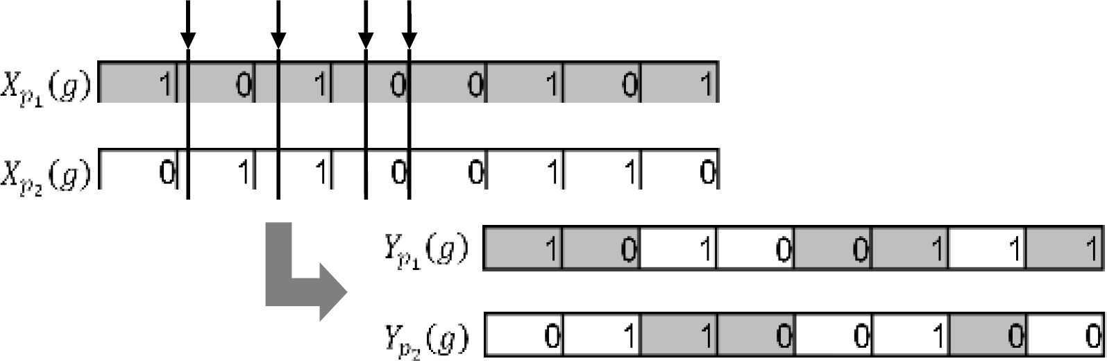
The chromosomes
Typically, this probability is set to 0.5, establishing uniform cut points [49]. Furthermore, this operator considers an additional parameter (
Mutation. The mutation randomly selects genes from a population of
where
In addition to the flipping operator, the cataclysmic mutation operator is also included, preserving the diversity of chromosomes through the restart procedure [50]. This operator is applied in the last generation of the GA, selecting the best chromosome from such generation.
Afterward, the remaining chromosomes are randomly generated to initialize a new population of
Stop condition. Once the GA has applied the genetic operators, it generates a new population of chromosomes. However, it requires iterating these operators several times to explore the search space. Typically, the GA runs until it reaches a certain number of generations (
5 Experiments and Results
This section is divided as follows: First, we present and describe the datasets used to evaluate summaries and select content measures. Second, we describe the configuration of evaluation measures employed for the proposed method. Third, we show the tuning of GA parameters that maximizes the correlation between the proposed selection of measures and human judgments. Fourth, we compare the performance of the proposed selection with state-of-the-art evaluation measures. Finally, we describe the analysis of the obtained results.
5.1 Datasets
To evaluate the performance of the proposed selection of measures, we have employed the DUC01 and DUC02 datasets. Indeed, previous studies suggest using these datasets because they have been widely used to generate and evaluate summaries [2, 3]. The DUC01 dataset contains 309 newspaper documents written in English, which are grouped into 30 collections. Each collection comprises 10 documents that address a particular topic (e.g., natural disasters, bibliographic information, etc.).
This dataset is commonly used for Single- and Multi-document summarization tasks of 100 words, leading to ATS systems being evaluated according to well-defined criteria. In particular, DUC01 holds 1776 summaries evaluated using
On the other hand, the DUC02 dataset contains 567 newspaper documents written in English, which are grouped into 59 collections. Each has between 5 and 12 documents addressing topics such as technology, food, politics, natural disasters, finances, etc. Like DUC01, this dataset is used for Single- and Multi-document summarization tasks of 100 words. In addition, DUC02 contains 4107 summaries evaluated through Coverage as a human judgment criterion [53].
5.2 Configuration of Evaluation Methods
According to the overall description of evaluation methods shown in Section “Evaluation Methods and Measures”, we have established certain parameters from them to generate several measures. Below, it is explained the configuration of each.
ROUGE-C. Besides eliminating stopwords and performing stemming, it is necessary to specify what measures were obtained from ROUGE-C. From ROUGE-C-N, we extracted n-grams from 1 to 5 to generate RC-1, 2, 3, 4, and 5, respectively. Furthermore, we employed Longest Common Subsequences (LCS) and skip-bigrams to obtain RC-L and RC-SU4, respectively.
LSA. The measures derived from the LSA depend on the combination of term-weighting formulas proposed in [35].
Based on this, 16 measures were generated from this method using the MTS (see Section “Evaluation Methods and Measures). Table 1 shows the name of each measure.
Table 1 LSA-based measures
|
Local Global |
FW | BW | AW | LW |
| NW | LSA-1 | LSA-2 | LSA-3 | LSA-4 |
| ISF | LSA-5 | LSA-6 | LSA-7 | LSA-8 |
| GF | LSA-9 | LSA-10 | LSA-11 | LSA-12 |
| EF | LSA-13 | LSA-14 | LSA-15 | LSA-16 |
FW: Frequency Weight, BW: Binary Weight, AW: Augmented Weight, LW: Logarithmic Weight, NW: No Weight, ISF: Inverse Sentence Frequency, GF: GFidf, and EF: Entropy Frequency.
SIMetrix. As mentioned in Section “Evaluation Methods and Measures”, the best measures of SIMetrix derive from
5.3 Tuning of GA Parameters
The GA parameters described in Section “Proposed Genetic Operators” are frequently used in other studies to adjust the performance of each genetic operator. Thus, we adjusted these parameters to improve the selection of evaluation measures described in the previous section. Table 2 shows the most representative tunings of GA parameters, where each was executed thrice. As observed, we have focused on modifying
Table 2 Tuning of GA parameters
| No. | ||||||
| 1 | 100 | 100 | 2 | 0.98 | 0.00175 | 3 |
| 2 | 300 | 800 | 2 | 0.98 | 0.00190 | 5 |
| 3 | 100 | 800 | 2 | 0.98 | 0.00190 | 3 |
| 4 | 100 | 200 | 2 | 0.98 | 0.00175 | 3 |
| 5 | 200 | 200 | 2 | 0.98 | 0.00175 | 3 |
| 6 | 200 | 200 | 2 | 0.98 | 0.00180 | 5 |
| 7 | 200 | 200 | 2 | 0.95 | 0.00190 | 5 |
| 8 | 200 | 500 | 2 | 0.90 | 0.00175 | 5 |
| 9 | 200 | 500 | 2 | 0.95 | 0.00175 | 5 |
| 10 | 200 | 500 | 2 | 0.97 | 0.00175 | 5 |
| 11 | 200 | 500 | 2 | 0.98 | 0.00175 | 5 |
| 12 | 200 | 500 | 2 | 0.98 | 0.00195 | 5 |
| 13 | 300 | 500 | 2 | 0.98 | 0.00175 | 3 |
| 14 | 300 | 500 | 2 | 0.98 | 0.00190 | 3 |
| 15 | 300 | 800 | 2 | 0.98 | 0.00190 | 3 |
| 16 | 500 | 800 | 2 | 0.98 | 0.00190 | 3 |
Regarding
For each experiment shown in Table 2, training and test sets were defined to evaluate the performance of the proposed GA under the Pearson (P), Spearman (S), and Kendall (K) correlations. Nevertheless, DUC01 and DUC02 do not explicitly consider both partitions of data.
Due to this, we have translated the documents of both datasets into Spanish using the Google Translate API, which is currently available in a Python library (https://pypi.org/project/ googletrans). After that, the English documents were used as a training set to optimize the selection of measures, and translated documents were used as a test set to evaluate the performance of the GA.
The translation of documents allows us to evaluate whether the proposed selection of measures is suitable for different languages. It is also necessary because neither DUC01 nor DUC02 provide enough evaluation data to test the proposed method. Previous studies [54] suggest translating documents as an alternative that seeks to preserve the performance of individual evaluation measures when datasets do not provide enough human judgment data.
Table 3 shows the correlation results between the proposed GA-based selection of measures and human judgments on the DUC01 dataset, considering the tuning of GA parameters shown in Table 1 and Table 2.
Table 3 Correlation results between the proposed selection of measures and human judgments (
| No. | English (Train) | Spanish (Test) | ||||
| P | S | K | P | S | K | |
| 1 | 0.4910 | 0.4784 | 0.3348 | 0.4675 | 0.4398 | 0.3071 |
| 2 | 0.5110 | 0.4850 | 0.3406 | 0.4287 | 0.4341 | 0.3040 |
| 3 | 0.4981 | 0.4803 | 0.3368 | 0.4624 | 0.4319 | 0.3013 |
| 4 | 0.5017 | 0.4731 | 0.3311 | 0.4390 | 0.4270 | 0.2980 |
| 5 | 0.5044 | 0.4851 | 0.3411 | 0.4671 | 0.4480 | 0.3131 |
| 6 | 0.4969 | 0.4731 | 0.3318 | 0.4585 | 0.4296 | 0.3008 |
| 7 | 0.5175 | 0.4886 | 0.3433 | 0.4502 | 0.4198 | 0.2923 |
| 8 | 0.4805 | 0.4694 | 0.3297 | 0.4569 | 0.4298 | 0.2996 |
| 9 | 0.5058 | 0.4864 | 0.3408 | 0.4492 | 0.4239 | 0.2948 |
| 10 | 0.5093 | 0.4866 | 0.3419 | 0.4654 | 0.4376 | 0.3054 |
| 11 | 0.4999 | 0.4777 | 0.3340 | 0.4463 | 0.4163 | 0.2907 |
| 12 | 0.5048 | 0.4800 | 0.3369 | 0.4435 | 0.4118 | 0.2869 |
| 13 | 0.5018 | 0.4787 | 0.3355 | 0.4561 | 0.4298 | 0.3005 |
| 14 | 0.5044 | 0.4813 | 0.3378 | 0.4476 | 0.4194 | 0.2917 |
| 15 | 0.5006 | 0.4964 | 0.3482 | 0.4118 | 0.3985 | 0.2764 |
| 16 | 0.5030 | 0.4813 | 0.3380 | 0.4440 | 0.4172 | 0.2898 |
Note: The best results are highlighted in bold.
According to the correlation results shown in Table 3, the performance of the proposed selection of measures in the English language (training set) is improved when we increment
However, we noticed higher correlation results by incrementing crossover probability and slightly reducing mutation probability. Finally, it is observed that the remaining experiments show lower correlation results.
Table 4 shows the correlation results between the proposed selection of measures and human judgments on the DUC02 dataset, considering the tuning of GA parameters shown in Table 1.
Table 4 Correlation results between the proposed selection of measures and human judgments (Coverage) on the DUC02 dataset, considering the tuning of GA parameters
| No. | English (Train) | Spanish (Test) | ||||
| P | S | K | P | S | K | |
| 1 | 0.6467 | 0.6171 | 0.4483 | 0.6396 | 0.6058 | 0.4393 |
| 2 | 0.6469 | 0.6176 | 0.4488 | 0.6385 | 0.6047 | 0.4383 |
| 3 | 0.6449 | 0.6136 | 0.4455 | 0.6412 | 0.6072 | 0.4405 |
| 4 | 0.6443 | 0.6102 | 0.4429 | 0.6409 | 0.6091 | 0.4419 |
| 5 | 0.6481 | 0.6193 | 0.4499 | 0.6257 | 0.5963 | 0.4317 |
| 6 | 0.6466 | 0.6142 | 0.4461 | 0.6271 | 0.5983 | 0.4334 |
| 7 | 0.6459 | 0.6151 | 0.4465 | 0.6363 | 0.6025 | 0.4365 |
| 8 | 0.6483 | 0.6204 | 0.4511 | 0.6346 | 0.6012 | 0.4354 |
| 9 | 0.6479 | 0.6196 | 0.4502 | 0.6221 | 0.5932 | 0.4292 |
| 10 | 0.6439 | 0.6123 | 0.4444 | 0.6211 | 0.5950 | 0.4319 |
| 11 | 0.6462 | 0.6127 | 0.4451 | 0.6323 | 0.6023 | 0.4371 |
| 12 | 0.6465 | 0.6153 | 0.4469 | 0.6305 | 0.6032 | 0.4372 |
| 13 | 0.6462 | 0.6198 | 0.4505 | 0.6320 | 0.5999 | 0.4346 |
| 14 | 0.6467 | 0.6148 | 0.4465 | 0.6257 | 0.5986 | 0.4337 |
| 15 | 0.6457 | 0.6124 | 0.4448 | 0.6326 | 0.6032 | 0.4374 |
| 16 | 0.6503 | 0.6220 | 0.4521 | 0.6281 | 0.5976 | 0.4330 |
Note: The best results are highlighted in bold.
Unlike previous correlation results, the best correlations are obtained when the parameters of the 4th experiment were employed (
On the other hand, we have observed that the proposed GA reaches higher correlation results in the training set when we improve exploration and intensification over the next experiments. However, the performance in the test set is reduced. That is, it produces overfitting. Therefore, focusing on exploration over exploitation is necessary because while selecting measures would be more specific, it is not generalizable.
Regarding complexity levels of content measures, Fig. 5 shows an overall ranking of complexity values obtained by the proposed GA to state-of-the-art evaluation measures. In particular, we have observed that the LSA-2, 7, 14, 3, 10, 1, and RC-1 have obtained the lowest complexity values in the ranking, which are lower than 0.1.
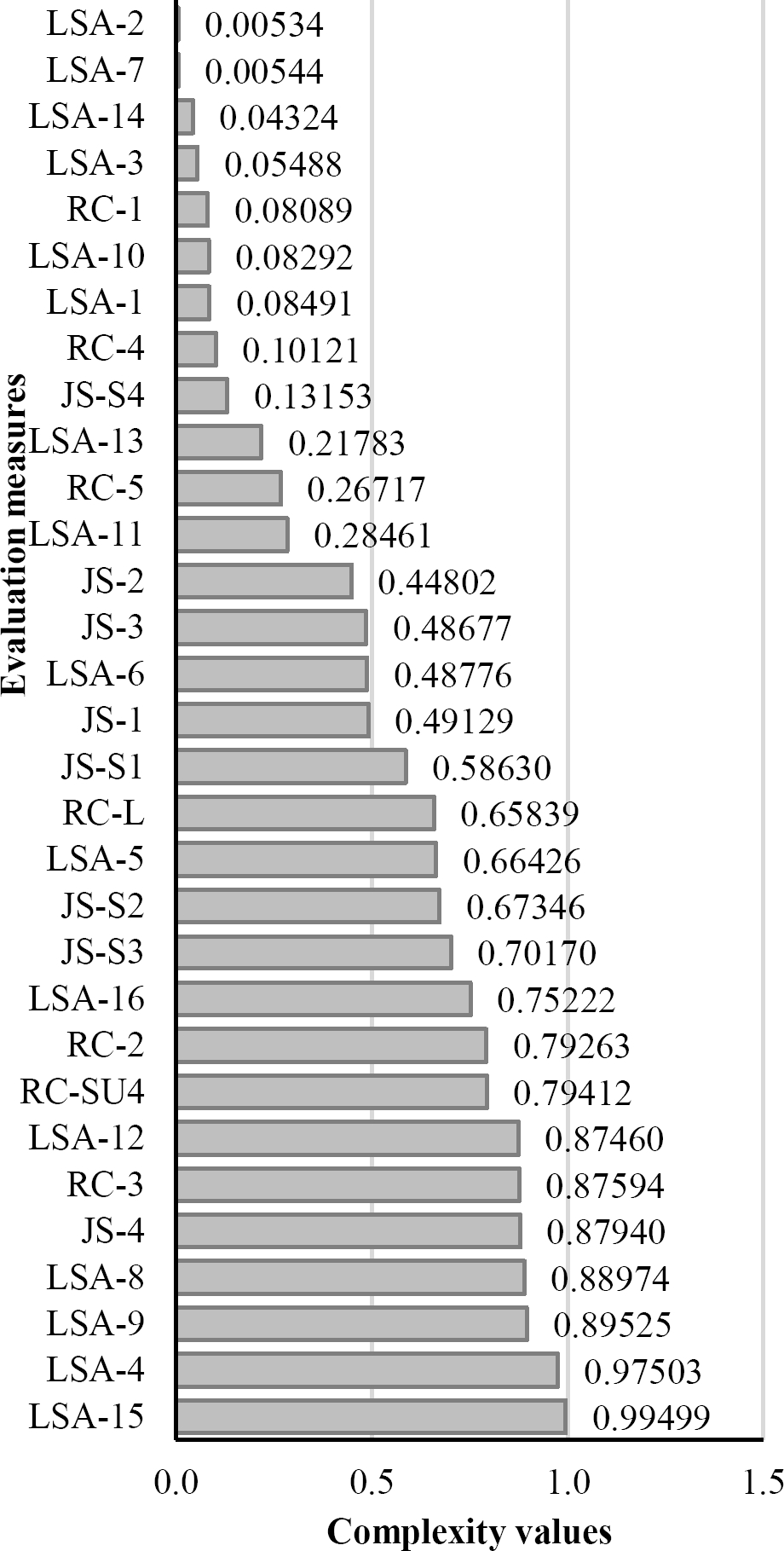
This lets us assume that these measures evaluate a small portion of summaries because their corresponding source documents have complexities lower than 0.1. Additionally, the following measures have obtained similar complexities: RC-4, JS-S4, LSA-13, RC-5, and LSA-11.
On the other hand, we noticed that the SIMetrix divergence measures, LSA-6, 5, and RC-L, have obtained higher complexity values, which in turn may indicate that these measures are more frequently selected to evaluate summaries. In other words, the complexity values of their corresponding source documents have achieved similar results.
Finally, it is worth mentioning that the remaining measures have obtained complexities near the highest complexity value possible (1.0). This is because some measures were selected because their source documents obtained similar complexities. Moreover, we have noticed that LSA-4 and LSA-15 were chosen not to evaluate any summary. It means that the proposed GA tends to exclude some measures, assigning them very high or low complexities implicitly.
From the above results, we have chosen the best correlation results (4th and 5th experiment) to compare the performance between the proposed selection of measures and state-of-the-art measures. Table 5 shows this comparison of DUC01 and DUC02 datasets translated into Spanish. The purpose of such a comparison is to highlight the importance of how the proposed selection of measures may be affected across a different language that is not English.
Table 5 Comparison between the proposed selection of measures and state-of-the-art evaluation measures
| Measure | DUC01 | DUC02 | ||||
| P | S | K | P | S | K | |
| Proposed | 0.4390 | 0.4270 | 0.2980 | 0.6409 | 0.6091 | 0.4419 |
| Proposed | 0.4671 | 0.4480 | 0.3131 | 0.6257 | 0.5963 | 0.4317 |
| SECO-SEVA | 0.4619 | 0.4250 | 0.2964 | 0.6472 | 0.6120 | 0.4452 |
| Avg (baseline) | 0.4401 | 0.4042 | 0.2800 | 0.6069 | 0.5691 | 0.4113 |
| 0.4674 | 0.4361 | 0.3040 | 0.6185 | 0.6189 | 0.4506 | |
| 0.4648 | 0.4338 | 0.3019 | 0.5452 | 0.6086 | 0.4402 | |
| LSA-3 | 0.4528 | 0.4182 | 0.2906 | 0.6426 | 0.6069 | 0.4402 |
| LSA-15 | 0.4575 | 0.4232 | 0.2944 | 0.6454 | 0.6106 | 0.4434 |
| LSA-11 | 0.4418 | 0.4087 | 0.2838 | 0.6402 | 0.6028 | 0.4373 |
Moreover, how individual measures (e.g.,
According to the obtained results, the proposed selection of measures has achieved the highest Spearman and Kendall correlation results on the DUC01 dataset, obtaining 0.4480 and 0.3131, respectively. Moreover, its performance on the Pearson correlation (0.4671) shows closeness to the highest result (0.4674). In general, these results suggest that the proposed selection improves automatic evaluation even if summaries and source documents are not in English. Moreover, it is worth mentioning that if we only consider the baseline approach, the results would be far from the best evaluation measures.
However, the performance of the proposed selection of measures is competitive with the best measures on the DUC02 dataset, obtaining P: 0.6409, S: 0.6091, and K: 0.4419. Compared to SECO-SEVA and
6 Conclusions and Future Works
In this paper, we propose a selection of content measures to evaluate summaries without human references using a Genetic Algorithm (GA). In addition, 12 text complexity indexes were used to measure source documents' degree of ease or difficulty (see Section “Text Complexity Indexes”). Moreover, we have proposed a GA that seeks to assign complexity values to content measures. The employed fitness function measures the correlation between the optimized selection of measures and human judgments.
According to the results obtained from several experiments, the proposed selection of measures achieves the best correlations on the DUC01 dataset, improving the evaluation of text summaries without human references. Despite the proposed selection of measures shows lower correlations to the best individual measures, it still shows competitive performance, showing proximity to the highest correlation results.
This also suggests that the selection of measures captures the strengths of several individual content measures. For this reason, we propose as future work the inclusion of other evaluation measures (e.g., MoverScore [55] or BERTScore [56]). In addition to this, we seek the inclusion of other text complexity indexes that may help to measure other aspects of complexity of source documents.
Finally, it is worth highlighting that using other GA operators and parameters may improve the process of exploration and intensification of the GA. Moreover, it would be useful using the proposed selection of measures to improve other NLP tasks such as ATS, and Text Classification.

